Before this: The transfer matrix.

Take a polynomial P and let x walk once round the unit circle, x = e^(i t) with t from 0 to 2 pi. At every point P(x) is a complex number with a size abs(P(x)), large in some places and zero at a root. The Mahler measure is the average of its logarithm, m(P) = (1/(2 pi)) integral_0^(2 pi) log abs(P(e^(i t))) dt. Some books use M(P) = e^(m(P)) instead, the geometric mean of the size.

The logarithm turns products into sums, so m(P Q) = m(P) + m(Q). Write P(x) = a (x - r_1) ... (x - r_d) with a the leading coefficient and r_1 to r_d the roots, and it is enough to know the measure of one factor x - r. A root inside the circle, or on it, costs nothing: on the circle abs(x - r) = abs(1 - r/x), and log abs(1 - r w) averaged over a circle of w equals its value at the centre, log 1 = 0. A root outside costs log abs(r), since x - r = -r (1 - x/r) and the second factor again averages to 0.

Add the factors and you have Jensen's formula, m(P) = log abs(a) + sum_k log max(1, abs(r_k)): the measure is the logarithm of the leading coefficient times the product of the roots outside the circle, and the roots inside are invisible. Mahler 1962 used the same average for polynomials in several variables, which is where the name comes from.

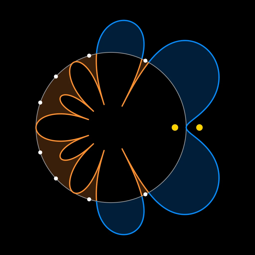
The figure is L(x) = x^10 + x^9 - x^7 - x^6 - x^5 - x^4 - x^3 + x + 1. The grey ring is the unit circle and the curve is log abs(L) drawn round it, standing out from the ring in blue where the size is above 1 and dipping inside in orange where it is below. At the eight roots on the circle the logarithm falls to minus infinity, so those dips are squeezed to stop short of the centre, each one on the ray of its root. The other two roots are the yellow dots, 0.85014 inside and 1.17628 outside. The true curve averages to log 1.17628 = 0.16236, the one root outside and nothing else.

Now let the coefficients be whole numbers. Then abs(a) >= 1 and every term is at least 0, so m(P) >= 0, with 0 only when a is plus or minus 1 and every root lies in the closed disc. Kronecker 1857 showed such roots are 0 or roots of one: the polynomial whose roots are the n-th powers of the roots has whole-number coefficients, bounded because the powers stay in the disc, so there are finitely many such polynomials and the powers repeat. So m(P) = 0 exactly when P is plus or minus a power of x times cyclotomic polynomials, those whose roots are roots of one: x - 1, x + 1, x^2 + x + 1, x^2 + 1 and so on. The roots of x^2 + x + 1 are the cube roots of one that build the Eisenstein integers.

How small can the measure be when it is not 0? Lehmer 1933 built large primes from the numbers (r_1^n - 1) ... (r_d^n - 1), which grow roughly like M(P)^n, so he wanted slow growth. The best he found was L, with M(L) = 1.17628.... Nobody has found smaller, and whether some fixed c > 0 bounds every nonzero measure of a whole-number polynomial from below is Lehmer's problem, still open. For an irreducible polynomial whose coefficients do not read the same backwards, even up to sign, it is settled: Smyth 1971 proved M(P) >= 1.3247..., the real root of x^3 - x - 1, unless P is plus or minus x. L reads the same backwards, which is why its roots come in pairs r and 1/r, like the two yellow dots. Smyth's survey collects the rest.

In several variables let x = e^(i s) and y = e^(i t) run round two circles independently, covering a torus, and average log abs(P(x, y)) over it. New numbers appear. Smyth 1981 found m(1 + x + y) = (3 sqrt(3) / (4 pi)) L(2, chi_-3) = 0.3230659..., where L(2, chi_-3) = 1 - 1/2^2 + 1/4^2 - 1/5^2 + 1/7^2 - ... skips the multiples of 3 and signs the rest by their remainder. That sign is the rule for whether a prime splits among the Eisenstein integers, and 1 + x + y vanishes on the torus only at x = omega, y = omega^2 and the swap. One variable more, m(1 + x + y + z) = 7 zeta(3) / (2 pi^2) = 0.4262783..., with zeta(3) a value of the Riemann zeta function. Boyd 1998 found by computer dozens of two-variable measures, such as those of x + 1/x + y + 1/y + k, that match rational multiples of L'(E, 0), a value attached to the elliptic curve E where the polynomial vanishes, to many digits; a few have been proved since, as in Rogers and Zudilin 2012.

There is a physical way to feel the number. Pick a phase theta evenly at random round the circle, read the size abs(P(e^(i theta))), do it again with a fresh phase n times in all, and multiply. The logarithm of the product is a sum of n independent draws, so by the law of large numbers that sum divided by n is close to m(P): the product grows like M(P)^n. Each factor is a one by one transfer matrix that depends on a phase, and m(P) is the Lyapunov exponent of their product, the growth per step of a typical run.

Typical is the key word. For P(x) = 1 + x the root -1 is on the circle, so m(P) = 0 and a typical product wanders without exponential growth. Yet abs(1 + e^(i theta))^2 averages to 2, the sum of the squared coefficients, so the mean square of the product doubles every step, carried by rare runs whose phases lean toward 0.

The same number is an entropy. A whole-number matrix with determinant plus or minus 1 moves the points of a torus without tearing it, and its entropy, the rate at which it pulls nearby points apart, is m(P) for P its characteristic polynomial: one log abs(r) for each eigenvalue that stretches. Lind, Schmidt and Ward 1990 proved the several-variable measure is the entropy of several commuting maps. A transfer matrix grows at its largest eigenvalue; the Mahler measure adds every eigenvalue that stretches.

In the tree

The fractal mirror note lays a stack of glass on a design, multiplies its layer matrices, and sets the drift of the stack against the Mahler measure of the design's digit polynomial and against a two-variable one. The transfer matrix gives the growth of one fixed table multiplied by itself; the Mahler measure is that growth averaged over a circle of tables. The two closed forms above lean on the Eisenstein integers and on the Riemann zeta function.