Before this: Fractal dimension.

A curve is what a pen draws without leaving the paper: it starts somewhere, moves without jumping, and stops somewhere. It seems obvious that such a line is thin and can never cover a patch of the plane. Peano 1890 showed that it can, by writing down a curve that passes through every point of a filled square. He did it with base-3 digits and no picture. A year later Hilbert 1891 gave a second one, built from a picture, and that picture is the recipe below.

Cut the square into four quarters and visit them along an arch: bottom left, top left, top right, bottom right. That arch is the motif, level 1, four cells and three steps. Now cut each quarter into four again and put a small copy of the arch in each, turned so that the end of one copy sits next to the start of the next. That is level 2, sixteen cells and fifteen steps. Keep going: at every level each cell is replaced by a scaled copy of the motif, four cells for one, and the copies are joined end to end. Level k visits 4^k cells in 4^k - 1 steps, never visits a cell twice and never lifts the pen.

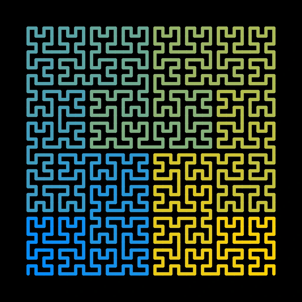
The figure is level 5: all 1024 cells of a 32 by 32 board visited in 1023 steps, tinted from blue where the walk starts, at the bottom left, to yellow where it ends, at the bottom right. The four big quarters are four copies of level 4, the two lower ones turned on their sides so that the walk enters and leaves along the bottom edge. Look inside any quarter and it is four copies again, and so on down to single cells.

Each level is still only a walk through cell centres. The space-filling curve is what the walks settle down to. Give the pen a clock that runs from 0 to 1, and at level k cut the clock into 4^k equal ticks, the i-th tick belonging to the i-th cell of the walk. Going one level deeper cuts every tick into four and every cell into four, and the four smaller ticks belong to the four smaller cells inside the old one. So a time t belongs to a chain of cells, each inside the last, shrinking to a single point, and that point is where the curve is at time t. Every point of the square sits in some such chain, so every point is reached. Two times less than one tick apart fall in the same cell or in two cells side by side, so their points are close: the curve never jumps. A map from the interval that is continuous and reaches every point of the square is exactly what space-filling means, and Sagan 1994 is the standard book on it.

The price is that the curve cannot be one-to-one: some points are reached at more than one time. This is forced. A continuous one-to-one map from an interval onto a square would have a continuous inverse, and removing one point cuts an interval in two but leaves a square in one piece. So every space-filling curve touches itself somewhere.

The counting also gives the dimension. Each level has four times as many steps, each half as long, so the curve is 4 copies of itself at half the size, and its fractal dimension is log 4 / log 2 = 2, the dimension of the square it fills. Peano's curve cuts the square into a 3 by 3 board instead and snakes through the nine cells, up the first column, down the second, up the third: 9 copies at a third of the size, and log 9 / log 3 = 2 again.

On a grid a walk of unit steps is described completely by its turns: after each step go straight, turn left or turn right. So the recipe can be written as a rewriting rule on letters. Hilbert's curve uses two letters A and B for the two mirror-image copies of the motif, F for a step forward and + and - for quarter turns left and right. Start from A and replace, all at once and at every level, each A by +BF-AFA-FB+ and each B by -AF+BFB+FA-. Five rounds of this, read by a pen that ignores A and B, draw the figure. Arndt 2016 searches rules of this kind systematically, one letter to replace and the rest turns, for curves that run along every edge of a grid once rather than through every cell. He finds all the small ones on the square, triangular and tri-hexagonal grids, and shows how to turn them into curves through every point of any uniform grid of the plane.

Nothing ties the idea to squares. On the triangular lattice of the Eisenstein integers a step can point in six directions a sixth of a turn apart. The Gosper curve, also called the flowsnake, replaces every step by seven steps. Measured in the new steps, the old one is a lattice vector of norm 7, such as 3 + omega, so each new step is shorter by the square root of 7, and 7 copies at that scale give dimension log 7 / log sqrt(7) = 2 once more. Its turns are sixths and thirds of a turn rather than quarters. The region its levels fill is no square but a hexagon with a crinkled edge, the Gosper island, and seven islands fit together into one larger island, turned a little and larger by the square root of 7.

What makes these curves useful is locality: points close together along the curve are close together in the plane. The clock argument above says how close. Halving the distance in the plane costs a factor of four in time, so the gap between two points of Hilbert's curve is at most a fixed multiple of the square root of the gap between their times. The converse fails. Two cells side by side can be far apart along the walk, and the figure shows one such place: at the bottom of the middle line, cells from early in the walk touch cells from late in it, blue against yellow.

That one-way locality is enough for a lot. A computer's memory is one long line of addresses, and it fetches neighbouring addresses together; store a grid, an image or a map in curve order and every small square patch lands in a few short runs of memory. Scan an image in curve order and successive pixels are always next to each other, which helps compression and the kind of dithering that passes an error on to the next pixel. A 3D printer fills the inside of each layer by following a path, and a curve like this fills a region in one stroke that stays near where it has just been, and some slicers offer a Hilbert infill. Every corner slows the print head, so how often a curve turns, and how sharply, is a practical question.

In the tree

The toolpaths note takes self-similar curves on the triangular lattice, the Gosper curve among them, as one-stroke print paths and counts how often they turn sharply. The radix dial reads the region the flowsnake fills as a radix tile, seven digits in a base of norm 7 on the Eisenstein integers, and the radix demo draws that tile as one of its presets. The dimension 2 of every curve here is the number fractal dimension reads off by counting boxes.